Introduction to ChIP-Seq

Overview

• Background
• Quality controls
• Read trimming and filtering
• Alignment
• Peak calling
• Peak calling using MACS
• Visual exploration
• Handling replicates
• Motif enrichment analysis
• Functional enrichment

This session provides a basic introduction to conducting a ChIP-seq analysis using the Galaxy framework. Some material has been borrowed Morgane Thomas-Chollier’s ChIP-seq tutorial and Galaxy workflow, and the Princeton HTSEQ Users Tutorial.

A pdf of step-by-step snapshots for these course materials is available here.

Course scope

We will be retracing most of the steps required to get from an Illumina FASTQ sequence file received from a sequencing facility as part of an ChIP sequencing analysis all the way to performing peak calling and identifying over represented sequence motifs and functional annotations. We will focus on the following steps: initial quality control, read mapping, peak calling, identification of over represented sequence motifs, annotation of regions with genes, and functional enrichment analysis of the peaks. Feel free to work through all examples and explore the reading material.

The default Galaxy instance relies on MACS for peak calls. Several other peak calling algorithms are also available in Galaxy; e.g., SICER has been specifically designed to for analysis of histone modifications and is available through the Galaxy Toolshed. For this exercise, we will use MACS to identify ChIP-seq peaks for two transcription factors and compare the results.

Requirements

Before tackling the modules below you should have a working knowledge of Galaxy, understand how to find relevant tools, annotate your history or get new data sets from the data library. As always, do ask questions and most importantly collaborate with your fellow students.

In order for you to be able to access Galaxy on your assigned dedicated machine on the Cloud, you have been given a web or IP address in the form of A.B.C.D where A, B, C and D are numbers separated by dots. You will find the current IP address at the top of our resource page. You will need it in order to access Galaxy from the web browser on your laptop.

If you want to work through this session outside of this course, take a look at our section on how to set up your own Galaxy server or download the complete introduction dataset and use one of the public Galaxy instances.

Background

We will ultimately be comparing the binding profiles of two transcription factors, Nanog and Pou5f1 (Oct4) from the HAIB TFBS ENCODE collection that have been ChIP-sequenced with Illumina in h1-ESC cells. Do look up the transcription factor (TF) information if you are not familiar with them as it should give you an idea what to expect in terms of TF binding.

To keep things manageable and allow algorithms to finish within a few minutes we will work with a single sample (“h1-hESC - Input replicate 1”), using reads from 32.8 Mb of chromosome 12 (chr12:1,000,000-33,800,000). We will switch over to using all samples to compare biological replicates and look at differential binding by different transcription factors by retrieving them from the Shared Data folders as needed.

Exploring the FASTQ files

Open up Galaxy from your machine as before, start up a new blank history and give it a name. In the top menu, move your mouse over Shared data and select Data libraries. This allows you to import files into Galaxy that have been shared with you.

Browse to the ChIP-Seq Data folder, expand the Sequence and reference data folder, and click on the arrow to the right of the filename H1hesc_Input_Rep1_chr12_unfiltered.fastq. In the context menu select Import this dataset into selected histories. On the next screen, select the history you are using. The file should now appear in your history

This is the kind of data you would expect to receive from your sequencing core facility: a large number of short nucleotide reads in FASTQ format (PDF).

Take a look at the file contents using Galaxy’s preview and file view functionality. What additional information does FASTQ contain over FASTA? How many reads are in your file? Pick the first sequence in your FASTQ file and note the identifier. What is the quality score of it’s first and last nucleotide, respectively?

Quality controls

The FASTQ file contains output reads from the sequencer that need to be mapped to a reference genome for us to understand where those reads came from on the sequenced genome. However, before we can delve into read mapping, we first need to make sure that our preliminary data is of sufficiently high quality. This involves several steps:

1. Obtaining summary quality statistics on the reads and review diagnostic graphs
2. Eliminate sequencing artifacts
3. Filter out genetic contaminants (primers, vectors, adaptors)
4. Filter out low-quality reads
5. Recalculate quality statistics and review diagnostic plots on filtered data

Iterate through steps 2-5 until the data is of sufficient quality before proceeding to mapping.

Obtain quality statistics

While Galaxy has a number of different methods to assess sequence properties you will want to stick to using a standard QC tool such as FASTQC in most cases.

Under the NGS: QC and manipulation tool find FASTQC: Read QC and give it a try.

What does the quality plot tell you about your data? What additional information do you get with this tool? What can you say about the per-base GC content? Does this match the human genome? Why is there a shift in the GC distribution from the theoretical distribution? Finally, what is the meaning of the k-mer content tab? This publication from Schroeder et al (PDF) has some background information.

Compare your results with a pre-generated FastQC plot obtained from the full FASTQ data set (i.e., using all reads).

Do you note any differences in the output or format? Why is that?

Some of the diagnostic plots from a Core conference call might be useful if you are curious to see what different modes of failure frequently look like.

Read trimming and filtering

Depending on your FASTQ results you may need to test for contamination (either by vector or other sources) and/or remove adapter sequences from your read prior to alignment. It is good to remove these sequences to increase your mapping efficiency. Note that this is not a problem for our sample data.

Screen for contamination

Not all required tools are available through Galaxy just yet. For example, depending on the source of your data you probably want to screen your reads for contamination using tools such as ContEst (PDF) or SeqTrim (PDF). For now we will just explore how you can spot potential contamination from the FastQC results alone.

What is the most overrepresented sequence in the pre-generated FastQC results from the h1-hESC sample?

Compare your own FastQC results with a different pre-generated FastQC summary that highlights a potential problem.

Study the report. Is there any vector contamination present? Is there any adapter contamination present?

As an emergency solution to remove contaminating sequences, Galaxy comes with a way to Clip adapter sequences. If you notice a particularly strong contamination with a vector or primer you can use your FASTQ file as the Library to clip, keep the default Minimum sequence length, and enter the sequence you spotted in the FASTQC report as the Adapter to clip. You probably want to keep both clipped and unclipped sequences in this case; keeping only reads that contained an adapter or barcode can be useful if you expect this to be a feature of all valid reads. For command-line use tools such as cutadapt are more versatile and less labor-intensive to use.

Normally, you would take the filtered output and feed it back into Galaxy, but our dataset has very little contamination so we will move on with the original data set.

Filter by quality

As we do not plan on using our data to identify genomic variation individual sequencing errors become less of a problem as long as the sequence can be still mapped to the reference genome. Still, you want to filter sequences where the overall quality is just too low.

After reviewing the quality diagnostics from your FASTQC report, choose an appropriate lower nucleotide quality that you think would be good for this data (for instance, a quality score below 20 means there is more than a 1/100 chance of an incorrect base call). Use this cutoff to filter out low-quality reads from your data with the Filter By Quality tool. After you have filtered your data generate another FASTQC quality report.

Do you have an improvement in read quality? What has changed and why? What percentage of reads did you retain at your cutoff?

Read trimming

After the general filtering which removes sequence reads of overall low quality it can be a good idea to trim the end of your reads, cutting away nucleotides at the end that are still of low-quality

Is this necessary in your case?

Use the Trim sequences tool to trim if required. Make sure to name your finalized FASTQ file that has been filtered and improved. You will be using this file in the next section for mapping. Again, tools such as sickle provide more flexibility by allowing for adaptive, window-based trimming, but are not yet part of the default Galaxy toolkit.

It might also be helpful to create a new history at this time and copy over your final sequence file. An easy way to do this is through the History menu and the Copy datasets function which allows you to pick one or more items in your current history, copying them over to a new or existing one.

Alignment

Next we are going to look at the steps we need to take once we have a clean, filtered FASTQ file that is ready for alignment. Use the filtered FASTQ file that you prepared in the previous section. The alignment process consists of the following steps:

• Choose an appropriate reference genome to map your reads against
• Choose an appropriate gene annotation model to guide your alignment
• Perform the read alignment

If for some reason any of the previous steps did not work you can retrieve a quality-controlled, trimmed and filtered FASTQ file from the Data Library in the ChIP-Seq Data library, subfolder Sequence and reference data (H1hesc_Input_Rep1_chr12_qualityfiltered.fastq).

Load the filtered FASTQ file and reference genome

To avoid excessive runtimes during later steps we will not align the reads against the whole human genome, just chr12:1,000,000-33,800,000. We have retrieved the sequence for this chromosome from UCSC GoldenPath (hg19) and added it to the “Data Library”. This means we won’t use the pre-built genome indices, but submit our own reference sequence. We are also using only a subset of reads from a single sample for the next few steps.

1. Start up a new blank history and give it a name.
2. Either load your filtered FASTQ files from the previous tutorial, or download a filtered FASTQ file from the Shared Data Libraries in Galaxy.
3. Find the chromosome 12 genomic sequence in the ChIP-Seq Data folder as hg19-chr12-reference_sequence.fa and import it into your new history.

Using it generates a slight time overhead since the reference genome needs to be indexed prior to each alignment run, but this is acceptable for now.

Perform read alignment

You will start by aligning your reads to chr12 using a standard aligner, Bowtie. If you’d like to learn more about its underlying algorithm, advantages and drawbacks a recent review from Bao et al (PDF) might be of interest. It also references the original paper which walks you through the methods.

You can find the tool under the NGS:Mapping tool heading. Make sure you select the corresponding tool for Illumina. Do not use the built-in reference genomes, and instead, select Use one from the history and choose the chr12-reference_sequence.fa. Select Single-End under “library mate pairing”. In the Bowtie settings, choose Full parameter list. As you can see, there are many parameters that you can change depending on the type of data you are working with. Change the Suppress all alignments for a read if more than n reportable alignments exist (-m) from -1 to 1 to ensure that only uniquely mapping reads are reported. Click the Execute button to launch the alignment. [Note: There’s also a Bowtie Version 2 by now, but we’ll stick to Bowtie 1 for the time being.]

While the alignment is running, do look up the documentation to see what the various tool options do. Take a look at the output file. Note it’s size. How long did it take to run? Now extrapolate to how long you would expect this tool to run when mapping to the entire genome (approximately).

Filter unmapped reads and convert SAM files to BAM files

Most aligners produce output in “SAM” format (Sequence Alignment/Map format by now, see publication from Heng Li (PDF) for more details).

Explore the SAM format. What key information is contained?

The SAM formatted output contains all reads along with flags indicating whether they have been mapped or not, their quality values and the genomic coordinates for mapped reads. Filter out the unmapped reads by applying the Filter SAM tool under NGS:SAM Tools. Click on the Add a new flag button. Select The read is unmapped under Type and set the state for this flag to No to discard unmapped reads.

How many lines are in this final file? This represents the number of aligned reads. Calculate the percentage of aligned reads for this experiment.

Another common preprocessing step for NGS data is to filter out duplicates. For ChIP-Seq data, these can be the result of a genuine signal or can be caused by PCR amplification artifacts, especially at high sequencing depth. Duplicates that result from ChIP enrichment form nice peaks surrounded by an otherwise more even distribution of reads. In general, the recommendation is to avoid directly filtering duplicates. MACS handles biases introduced by amplification and library preparation by removing duplicate reads if their count is higher than can be expected from the sequencing depth (binomial distribution with a p-value < 10e-05).

To speed up processing those need to get converted into their binary counterpart (BAM).

• Apply the SAM-to-BAM tool under the NGS:SAM Tools heading to convert your output SAM file to the compressed BAM format, once again using the chromosome 12 reference sequence from your history as reference

Explore alignment in a genome browser

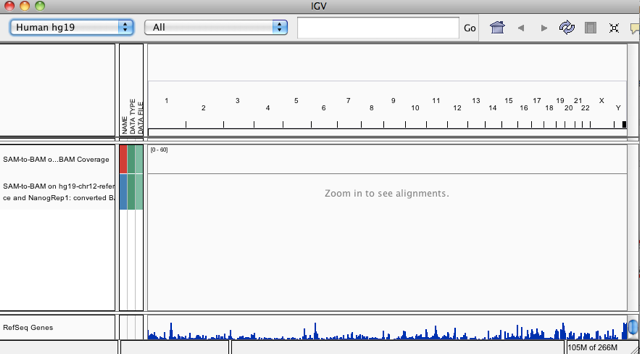
Take a look at your alignment in IGV (Integrative Genomics Viewer). To do so, first expand the alignment result (the BAM file) in your history and click on the web current link beside display with IGV. This will download IGV to your machine. It should start automatically after a few security warnings (if not, find the igv.jlnp file and click it yourself).

You should see a window that looks like this:

Click in the highlighted window…

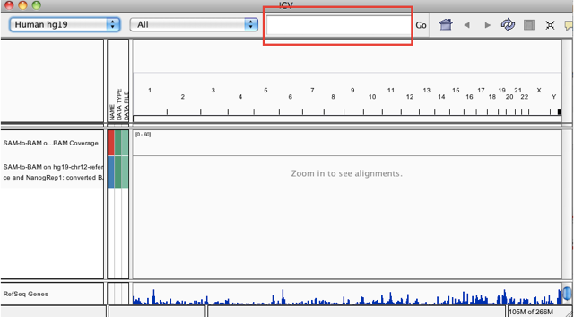
… and enter the gene name AKAP3. You should now be able to see the individual reads, you can zoom in further using the controls on the upper right and scroll around by clicking and dragging in the highlighted alignment track. Note that IGV automatically translated the gene symbol into the matching genomic coordinates for your genome build:

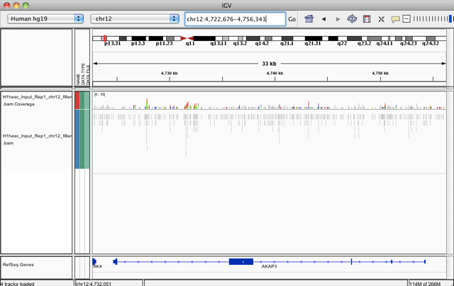
Recall that this is the input file, i.e. the control.

Can you identify any potential regions of enrichment in this gene or others?

ChIP-seq data is not distributed evenly across the genome and, even in the input sample, you will see clustering of reads around gene regions and especially around promoter areas, which is why we need the input/control sample. By comparing the number and distribution of reads between input and your sample, you essentially correct for this background read distribution.

Let’s compare the input and the corresponding Nanog TF ChIP-Seq data side by side, and this will be immediately apparent.

• Go to Shared Data, Data Libraries, open the ChIP-Seq Data folder, then open the Additional Sample data folder. Find the Nanog alignment data H1hesc_Nanog_Rep1_chr12_aln.bam and import it into your current history.

Expand the alignment result (the BAM file) in your history by clicking on the file name and then click on the local link beside display with IGV. This will automatically download the alignment file into the IGV window that is already open so you can compare the two alignment files.

Can you identify any potential Nanog binding sites based on the comparison of the input vs. Nanog ChIP results?

Peak calling

As before, if any of the previous steps did not work out you can retrieve intermediate results from the “Snapshot” Data Library under “Shared Data”. We have deposited the Bowtie-aligned reads in BAM format in the Additional sample data library.

The goal of peak calling is to define regions with a high density of reads indicating where the studied factor bound. There are multiple algorithms to perform the peak-calling step. In this workshop we will be using a tool called MACS.

ChIP signal strength is a continuum with far more weak sites than strong. As a result, the composition of the final peak list depends heavily on the specific parameter settings and algorithm as well as the quality of the experiment itself. Thresholds that are too relaxed lead to a high proportion of false positives for each replicate, but as you will see in the Handling Replicates section, subsequent analysis can remove false positives from a final joint peak determination.

Peak calling using MACS

We will use MACS to call “Nanog” peaks in a ChIP (tag) sample versus a control (input) sample. Although MACS can be run without a control data set, an appropriate control is critical for robust analysis of any ChIP-seq experiment because DNA breakage during sonication is not uniform. Some regions of the genome, particularly those at open chromatin, are sheared more readily than others and these fragments can be over-represented in the sequencing step, giving rise to false positive sites of occupancy. The control data set for this study used DNA isolated from cells that were cross-linked and fragmented under the same conditions as the ChIP DNA but without the antibody. This is sometimes referred to as “reverse-cross-linked chromatin” or “Input DNA”. An alternative approach is a “mock IP” in which a control antibody IgG antibody is used that does not recognize any DNA binding protein (“IgG” control). Additional information can be obtained from the ENCODE/modENCODE ChIP-seq guidelines.

1. Copy the aligned control (input) BAM file and the H1hesc_Nanog_Rep1_chr12_aln.bam from the previous section to a new history.
2. Select MACS from the NGS:Peak Calling menu.
3. Enter an Experiment Name (e.g., MACS_NanogRep1)
4. Select the H1hesc_NanogRep1_chr12_aln.bam file for the ChIP-Seq Tag File, and the H1hesc_InputRep1_chr12_aln.bam file for your ChIP-Seq Control File.
5. Note the Effective genome size, which is the size of the genome that is can be sequenced and mapped (minus telomeres, repeats, etc). Use the default since we are dealing with human data (2,700,000,000). For mouse, the value is 1,870,000,000. For less commonly used species, an estimate of 70-90% of the full genome size is reasonable.
6. Set the Tag size to 36bp (based on examining the FastQC report).
7. Note the Band width parameter. This value is used to scan the genome for model building. You can set this parameter as the expected sonication fragment size. We will leave it at the default value of 300.
8. Note the MFOLD parameter which is used to select genomic regions to build the experiment-specific peak model. A region is used for the model if it contains more than mfold reads than the region surrounding it. We will use the default value (32) but this value can be tweaked to obtain more or less peaks.
9. Check the box for Perform the new peak detection method (futurefdr). This uses both the control and treatment data to calculate local bias and identify peak locations.

While MACS is running, use the time to browse through its manual or explore the MACS Protocol paper (PDF) which describes how to set parameters for transcription factor binding and histone modification data sets, and how to interpret the output. A new version, MACS2 is available, but we will be using the older version for today’s exercises.

The algorithm will generate two files. The first output is a BED file with the coordinates of the peaks. Instructions for viewing the peaks in IGV follows below.

How many peaks (“regions”) were detected by MACS?

The second output is an HTML page that links to the results in various formats and lists the parameters and tasks that were performed. Although warning messages do not affect the success of a MACS run, the majority should still be carefully evaluated. For example, the warning message ‘Treatment tags and Control tags are uneven’ means that the FDR of the resulting peaks will be overestimated when the control sample has more reads and will be underestimated when the ChIP-seq sample is sequenced more deeply. The message ‘Fewer paired peaks X than 1,000’ means that MACS only identified X model peaks and may indicate potential data quality issues because 1,000 model peaks are needed to robustly estimate ChIP-DNA fragment size. The message ‘missing chromosome X data’ might suggest that the raw input file for that chromosome is incomplete.

Under Additional Files, click on the first file ending with model.pdf. This file shows the peak model built by MACS. ChIP-Seq DNA fragments are sequenced from the 5’ end, resulting in alignment of tags that form two peaks, on each strand, flanking the location that was bound by the protein of interest. The red curve represents the distribution of reads on the positive strand at each base position, and the blue line models the reads on the negative strand. The black curve is the combined profile that is generated by shifting each distribution toward the center. The detected DNA fragment length is given by d and varies among different ChIP-seq libraries.

Note that the estimated fragment length (d) is 103 which is much smaller than the default band width parameter of 300 used by MACS. This accounts for the jagged peak model. If you run it again and modify the band width parameter to 100, you will see smooth peaks in the peak model diagram.

The peaks.xls file contains all of the information about the peaks identified by MACS, including key parameters, coordinates and enrichment statistics.

Visual exploration

We will use IGV again to study some of the results:

1. View the resulting MACS peaks: bed file in IGV. As Galaxy does not support automatic export of BED files to IGV, you will have to add it to IGV yourself. To do so, download the file from Galaxy and take note of where you saved it. Now move over to IGV and click the File menu and then Load from file. Select the file you downloaded and open it in IGV to explore the MACS peak calls next to your Bowtie alignment.
2. Type Akap3 in the coordinate text box to zoom in on this region and observe the correlation between the MACS peak call and the alignment. Another interesting gene to look at is Sox5.

Handling replicates

In your own analyses, you will have multiple conditions and (hopefully!) multiple replicates for those conditions. Technical replicates are usually merged after FASTQC analysis to ensure that the sequencing quality is adequate. FastQ files can be concatenated at the read level or BAM files can be merged after alignment using SAMtools.

Biological replicates should be analyzed individually first and then compared at the peak call level. Key questions to ask are whether replicates correlate well and if there is substantial peak overlap. The current state-of-the-art for analyzing ChIP-Seq replicates and setting thresholds is the Irreproducible Discovery Rate (IDR), which compares a pair of ranked lists of peaks and creates a curve to quantitatively determine the extent to which the ranks are no longer consistent across the replicates. The method was developed and used extensively for the ENCODE and modENCODE projects and is part of their ChIP-seq guidelines. The method is not yet available in the standard Galaxy installation, however.

In the meantime, there are simple things in Galaxy that you can do to analyze replicates and additional samples, such as intersecting and subtracting peaks to get common and unique regions in two samples.

Bringing in replicates and another sample

Up to now we have been analyzing a single ChIP experiment (Nanog-Rep1-chr12 sample and Input-Rep1-chr12 control) to save time. Now we will bring three other ENCODE data sets into our analysis. We have generated the necessary files – the second H1Hesc Nanog replicate and two replicates for H1Hesc Pou5f1 (Oct4) – for you and placed them in the Shared Data Library under ChIP-Seq Data; they can be found in the Additional Sample Data folder. Open up this folder and import the following peak calls for each of the other 3 ENCODE samples to your history (making sure to specify the bed format):

• MACS_Nanog_Rep2.chr12.bed
• MACS_Pou5f1_Rep1.chr12.bed
• MACS_Pou5f1_Rep2.chr12.bed

To increase our confidence in the peak calls, we will combine our replicate files and take the intersection of the two. Click on Operate on Genomic Intervals and Concatenate the two Nanog replicates to combine them into one file. Next, use the Cluster tool on the concatenated data to combine overlapping peak calls using the default parameters.

How many peaks are retained? What fraction of the individual replicates are retained?

A simple heuristic used by the ENCODE project prior to IDR was to retain replicates for analysis if either 80% of the top 40% of identified targets in one replicate were among the targets in the second replicate; or 75% of target lists were in common between both replicates.

Note that the resulting peak calls are dominated by the “weakest” replicate. You will probably have noticed that there is also an Intersect tool and may be wondering why we did not use it directly on the two replicates. If we had, only peaks in the first replicate that overlap with the second would be returned, i.e. overlapping regions would not be merged to form a larger region encompassing the coverage from both replicates.

Repeat these steps for the Pou5f1 replicates to prepare to look for differential enrichment of binding sites.

Differential binding

To identify sites that have differential binding, across two conditions, developmental stages, factors, etc., we will use Galaxy’s Subtract tool on the intersected peak calls for Nanog and Pou5f1. Select the clustered Pou5f1 file for the first input and the clustered Nanog file for the second input, and return intervals with no overlap. The resulting dataset contains regions where Nanog binds but Pou5f1 does not. You can then switch the inputs to find regions where Pou5f1 binds but Nanog does not.

Note: You can also use MACS directly to find differential binding between two conditions by treating one of the samples as the control.

Find regions where both TFs bind using the approach above for intersecting two replicates.

Motif and functional enrichment analyses are unlikely to give reliable results given that you are only looking at 32.8 Mb of reads mapping to chr12. To obtain more signal, we will use the complete set of Nanog peak calls generated by ENCODE and look at binding sites for the whole of chr12. This will also keep the sequence data size manageable for this tutorial.

Motif enrichment analysis

Start by importing Encode-hesc-Nanog.narrowPeak from the Galaxy “Data Library” in the “ENCODE peak calls” folder. It is in narrowPeak format and contains Nanog peak calls for the whole genome. The format is an extension of the BED format and was developed to describe peaks of signal enrichment for pooled, normalized data.

Convert this file to BED format by editing the attributes and selecting the Convert Format tab. Select Convert Genomic Intervals to BED and click Convert.

To perform motif enrichment, we need to retrieve the genomic DNA sequences for the set of peaks. To do this, you will also need the hg19-chr12-reference_sequence.fa we used previously for the alignments. Import this file into your current history from either a previous history or the Data Library. Recall that it was located in Sequence and reference data in the Shared Data library.

1. Click on Fetch Sequences followed by Extract Genomic DNA.
2. Select the Encode-Nanog.narrowPeak file.
3. Change the Source for Genomic Data to History, and then select hg19-chr12-reference_sequence.fasta.
4. Click Execute to generate a FASTA file containing the genomic DNA given by the coordinates in the file.

Note that only the chr12 regions are generated because we used the chr12 reference sequence. Download this file to your computer for use in the motif over-representation analysis.

To identify over-represented motifs, we will use DREME from the MEME suite of sequence analysis tools. DREME is a motif discovery algorithm designed to find short, core DNA-binding motifs of eukaryotic transcription factors and is optimized to handle large ChIP-seq data sets.

1. Visit the DREME website and select the downloaded Nanog peaks as input to DREME
2. Enter your email address so that DREME can email you once the analysis is complete
3. Enter a job description so you will recognize which job has been emailed to you and then start the search.

You will be shown a status page describing the inputs and the selected parameters, as well as a link to the results at the top of the screen. Clicking the link displays an output page that is continually updated until the analysis has completed. DREME will also email you once the analysis is complete. This may take some time depending on the server load and the size of the file. While you wait, take a look at the expected result (obtained by clicking on the HTML output link once the analysis has completed).

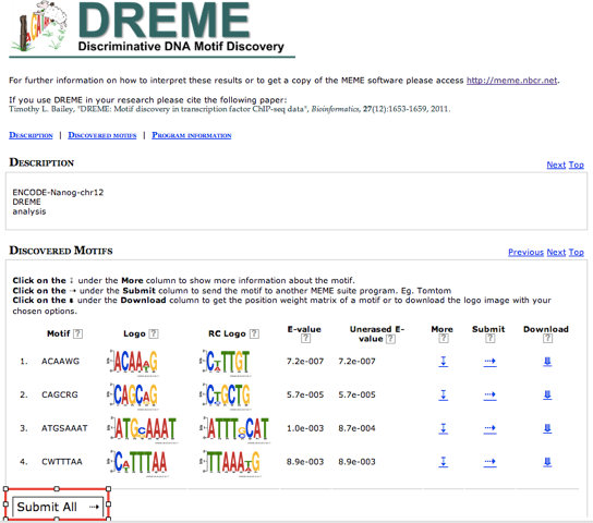
DREME’s HTML output provides a list of Discovered Motifs displayed as sequence logos (in the forward and reverse complement (RC) orientations), along with an E-value for the significance of the result. Clicking on More displays the number of times the motif was identified.

To determine if the identified motifs resemble the binding motifs of known transcription factors, we can submit them to Tomtom, which searches a database of known motifs to find potential matches and provides a statistical measure of motif-motif similarity. We can run the analysis individually for each motif prediction, or analyze them all at once.

1. Scroll to the bottom of the motif list and click Submit All. A dialog box will appear asking you to Select what you want to do or Select a program. Select Tomtom and click Send.
2. This takes you to the input page. Tomtom allows you to select the database you wish to search against. We will use the default but keep in mind that there are other options when performing your own analyses.
3. Enter your email address and job description and start the search.

You will be shown a status page describing the inputs and the selected parameters, as well as a link to the results at the top of the screen. Clicking the link displays an output page that is continually updated until the analysis has completed. Like DREME, Tomtom will also email you the results.

The HTML output for Tomtom shows a list of possible motif matches for each DREME motif prediction generated from your Nanog regions. Clicking on the match name shows you an alignment of the predicted motif versus the match.

What are the possible identities for the motifs you discovered from the Nanog ChIP regions on chr12? Do these make sense given what you know about the Nanog transcription factor? Compare your results to results for the full ENCODE data set available from FactorBook and take a look at a Nanog binding matrix (from Ferraris et. al., 2013).

Functional enrichment

A large number of methods and external tools are available to make sense of a gene list, most of which revolve around detecting functional enrichment in Gene Ontology, curated pathways or networks. A recent post on Getting Genetics Done should get you started, and we will expand this section for future workshops. For now we will explore one approach that cover the basics.

In order to be able to identify functional enrichment we need to look at genome wide signals; instead of just looking at the ENCODE Nanog peak calls for chromosome 12 we will use the full set of calls. We will use GREAT to perform a functional enrichment. GREAT takes a list of regions, associates them with nearby genes, and then analyzes the gene annotations to assign biological meaning to the data:

1. Go back to Galaxy and download the BED file you created from the Encode-Nanog.narrowPeak file for the motif analysis. Make sure it is the BED formatted file as this is a requirement for the next step.
2. First select Human: GRCh37 (UCSC hg19, Feb/2009) for the Species Assembly.
3. Choose the ENCODE-Nanog.bed file and use the Whole genome for Background regions.
4. Click Submit.

GREAT provides the output in HTML format organized by section.

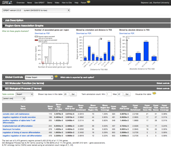
The first section contains the Job Description detailing the inputs and parameters. The Region-Gene Association Graphs indicate the number of associated genes per region, and the distances of the regions to transcription start sites (TSS), providing insights into the genomic organization of Nanog ChIP regions.

Explore the rest of the results. The output contains enrichment of GO terms, pathway / disease enrichments, miRNA and TF-targets. It is also worthwhile to click on the enriched annotation names to get a more detailed view of genes annotated with these terms.

---